4.3 Ionic and total abundances from CELs

We determined abundances for ionic species of N, O, Ne, S and Ar from CELs. To deduce ionic abundances, we solve the statistical equilibrium equations for each ion using EQUIB code, giving level population and line sensitivities for specified $N_{\rm e}=1000$ cm${}^{-3}$ and $T_{\rm e}=10\,000$ K adopted according to our photoionization modelling. Once the equations for the population numbers are solved, the ionic abundances, X${}^{i+}$/H${}^{+}$, can be derived from the observed line intensities of CELs as follows:

$$\frac{N({\rm X}^{i+})}{N({\rm H}^{+})}=\frac{I(\lambda_{ij})}{I({... ...)}{4861} \frac{\alpha_{\rm eff}({{\rm H}\beta})}{A_{ij}} \frac{N_{\rm e}}{n_i},$$ (2)

where $I(\lambda_{ij})$ is the dereddened flux of the emission line $\lambda_{ij}$ emitted by ion ${\rm X}^{i+}$ following the transition from the upper level $i$ to the lower level $j$, $I({{\rm H}\beta})$ the dereddened flux of H$\beta$, $\alpha_{\rm eff}({{\rm H}\beta})$ the effective recombination coefficient of H$\beta$, $A_{ij}$ the Einstein spontaneous transition probability of the transition, $n_i$ the fractional population of the upper level $i$, and $N_{\rm e}$ is the electron density.

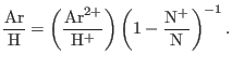
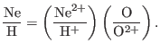
Total elemental and ionic abundances of nitrogen, oxygen, neon, sulphur and argon from CELs are presented in Table 7. Total elemental abundances are derived from ionic abundances using the ionization correction factors ($icf$) formulas given by Kingsburgh & Barlow (1994). The total O/H abundance ratio is obtained by simply taking the sum of the O$^{+}$/H$^{+}$ derived from [O II] $\lambda\lambda$3726,3729 doublet, and the O$^{2+}$/H$^{+}$ derived from [O III] $\lambda\lambda$4959,5007 doublet, since HeII $\lambda$4686 is not present, so O${}^{3+}$/H${}^{+}$ is negligible. 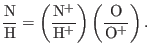The total N/H abundance ratio was calculated from the N$^{+}$/H$^{+}$ ratio derived from the [N II] $\lambda\lambda$6548,6584 doublet, correcting for the unseen N$^{2+}$/H$^{+}$ using,

$$\footnotesize \frac{{\rm N}}{{\rm H}}=\left(\frac{{\rm N}^{+}}{{\rm H}^{+}}\right) \left(\frac{{\rm O}}{{\rm O}^{+}}\right).$$ (3)

The Ne$^{2+}$/H$^{+}$ is derived from [Ne III] $\lambda$3869 line. Similarly, the unseen Ne$^{+}$/H$^{+}$ is corrected for, using

$$\frac{{\rm Ne}}{{\rm H}}=\left(\frac{{\rm Ne}^{2+}}{{\rm H}^{+}} \right) \left(\frac{{\rm O}}{{\rm O}^{2+}}\right) .$$ (4)

For sulphur, we have S$^{+}$/H$^{+}$ from the [S II] $\lambda\lambda$6716,6731 doublet and S$^{2+}$/H$^{+}$ from the [S III] $\lambda$9069 line. The total sulphur abundance is corrected for the unseen stages of ionization using

$$\footnotesize \frac{{\rm S}}{{\rm H}}=\left(\frac{{\rm S}^{+}}{{\... ...} \right) \left[1-\left(1-\frac{{\rm O}^{+}}{{\rm O}}\right)^{3}\right]^{-1/3}.$$ (5)

The [Ar III] 7136 line is only detected, so we have only Ar$^{2+}$/H$^{+}$. The total argon abundance is obtained by assuming Ar$^{+}$/Ar = N$^{+}$/N:

$$\footnotesize \frac{{\rm Ar}}{{\rm H}}=\left(\frac{{\rm Ar}^{2+}}{{\rm H}^{+}} \right) \left(1-\frac{{\rm N}^{+}}{{\rm N}}\right)^{-1}.$$ (6)

As it does not include the unseen Ar$^{3+}$, so the derived elemental argon may be underestimated.

Figure: Ionic abundance maps of Abell 48. From left to right: spatial distribution maps of singly ionized Helium abundance ratio He${}^{+}$/H${}^{+}$ from HeI ORLs (4472, 5877, 6678); ionic nitrogen abundance ratio N${}^{+}$/H${}^{+}$ ( $\times 10^{-5}$) from $[$N II$]$ CELs (5755, 6548, 6584); ionic oxygen abundance ratio O${}^{2+}$/H${}^{+}$ ( $\times 10^{-4}$) from $[$O III$]$ CELs (4959, 5007); and ionic sulphur abundance ratio S${}^{+}$/H${}^{+}$ ( $\times 10^{-7}$) from $[$S II$]$ CELs (6716, 6731). North is up and east is towards the left-hand side. The white contour lines show the distribution of the narrow-band emission of H$\alpha$ in arbitrary unit obtained from the SHS.

Fig.4 shows the spatial distribution of ionic abundance ratio He${}^{+}$/H${}^{+}$, N${}^{+}$/H${}^{+}$, O${}^{2+}$/H${}^{+}$ and S${}^{+}$/H${}^{+}$ derived for given $T_{\rm e}=10000$K and $N_{\rm e}=1000$cm$^{-3}$. We notice that both O${}^{2+}$/H${}^{+}$ and He${}^{+}$/H${}^{+}$ are very high over the shell, whereas N${}^{+}$/H${}^{+}$ and S${}^{+}$/H${}^{+}$ are seen at the edges of the shell. It shows obvious results of the ionization sequence from the highly inner ionized zones to the outer low ionized regions.

Table 7: Empirical ionic abundances derived from CELs.

Ion	$\lambda$(Å)	Mult	Value $^{\mathrm{a}}$
N${}^{+}$	6548.10	F1	1.356($-5$)
	6583.50	F1	1.486($-5$)
	Mean		1.421($-5$)
	$icf$(N)		3.026
N/H			4.299($-5$)
O${}^{+}$	3727.43	F1	5.251($-5$)
O${}^{2+}$	4958.91	F1	1.024($-4$)
	5006.84	F1	1.104($-4$)
	Average		1.064($-4$)
	$icf$(O)		1.0
O/H			1.589($-4$)
Ne${}^{2+}$	3868.75	F1	4.256($-5$)
	$icf$(Ne)		1.494
Ne/H			6.358($-5$)
S${}^{+}$	6716.44	F2	4.058($-7$)
	6730.82	F2	3.896($-7$)
	Average		3.977($-7$)
S${}^{2+}$	9068.60	F1	5.579($-6$)
	$icf$(S)		1.126
S/H			6.732($-6$)
Ar${}^{2+}$	7135.80	F1	9.874($-7$)
	$icf$(Ar)		1.494
Ar/H			1.475($-6$)

$^{\mathrm{a}}$

Assuming $T_{\rm e}=10\,000$K and $N_{\rm e}=1000$ ${\rm cm}^{-3}$.